Image Compression with Neural Networks
September 29, 2016
Posted by Nick Johnston and David Minnen, Software Engineers
Data compression is used nearly everywhere on the internet - the videos you watch online, the images you share, the music you listen to, even the blog you're reading right now. Compression techniques make sharing the content you want quick and efficient. Without data compression, the time and bandwidth costs for getting the information you need, when you need it, would be exorbitant!
In "Full Resolution Image Compression with Recurrent Neural Networks", we expand on our previous research on data compression using neural networks, exploring whether machine learning can provide better results for image compression like it has for image recognition and text summarization. Furthermore, we are releasing our compression model via TensorFlow so you can experiment with compressing your own images with our network.
We introduce an architecture that uses a new variant of the Gated Recurrent Unit (a type of RNN that allows units to save activations and process sequences) called Residual Gated Recurrent Unit (Residual GRU). Our Residual GRU combines existing GRUs with the residual connections introduced in "Deep Residual Learning for Image Recognition" to achieve significant image quality gains for a given compression rate. Instead of using a DCT to generate a new bit representation like many compression schemes in use today, we train two sets of neural networks - one to create the codes from the image (encoder) and another to create the image from the codes (decoder).
Our system works by iteratively refining a reconstruction of the original image, with both the encoder and decoder using Residual GRU layers so that additional information can pass from one iteration to the next. Each iteration adds more bits to the encoding, which allows for a higher quality reconstruction. Conceptually, the network operates as follows:
- The initial residual, R[0], corresponds to the original image I: R[0] = I.
- Set i=1 for to the first iteration.
- Iteration[i] takes R[i-1] as input and runs the encoder and binarizer to compress the image into B[i].
- Iteration[i] runs the decoder on B[i] to generate a reconstructed image P[i].
- The residual for Iteration[i] is calculated: R[i] = I - P[i].
- Set i=i+1 and go to Step 3 (up to the desired number of iterations).
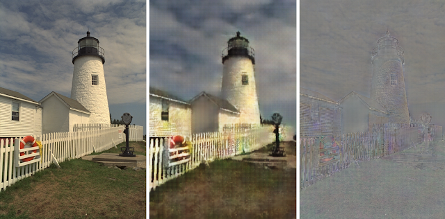
To understand how this works, consider the following example of the first two iterations of the image compression network, shown in the figures below. We start with an image of a lighthouse. On the first pass through the network, the original image is given as an input (R[0] = I). P[1] is the reconstructed image. The difference between the original image and encoded image is the residual, R[1], which represents the error in the compression.
 |
| Left: Original image, I = R[0]. Center: Reconstructed image, P[1]. Right: the residual, R[1], which represents the error introduced by compression. |
 |
| The second pass through the network. Left: R[1] is given as input. Center: A higher quality reconstruction, P[2]. Right: A smaller residual R[2] is generated by subtracting P[2] from the original image. |
To demonstrate file size and quality differences, we can take a photo of Vash, a Japanese Chin, and generate two compressed images, one JPEG and one Residual GRU. Both images target a perceptual similarity of 0.9 MS-SSIM, a perceptual quality metric that reaches 1.0 for identical images. The image generated by our learned model results in an file 25% smaller than JPEG.
 |
| Left: Original image (1419 KB PNG) at ~1.0 MS-SSIM. Center: JPEG (33 KB) at ~0.9 MS-SSIM. Right: Residual GRU (24 KB) at ~0.9 MS-SSIM. This is 25% smaller for a comparable image quality |
 |
| Left: Original. Center: JPEG. Right: Residual GRU. |
-
Labels:
- Machine Perception
- Product
Other posts of interest
-
April 19, 2024
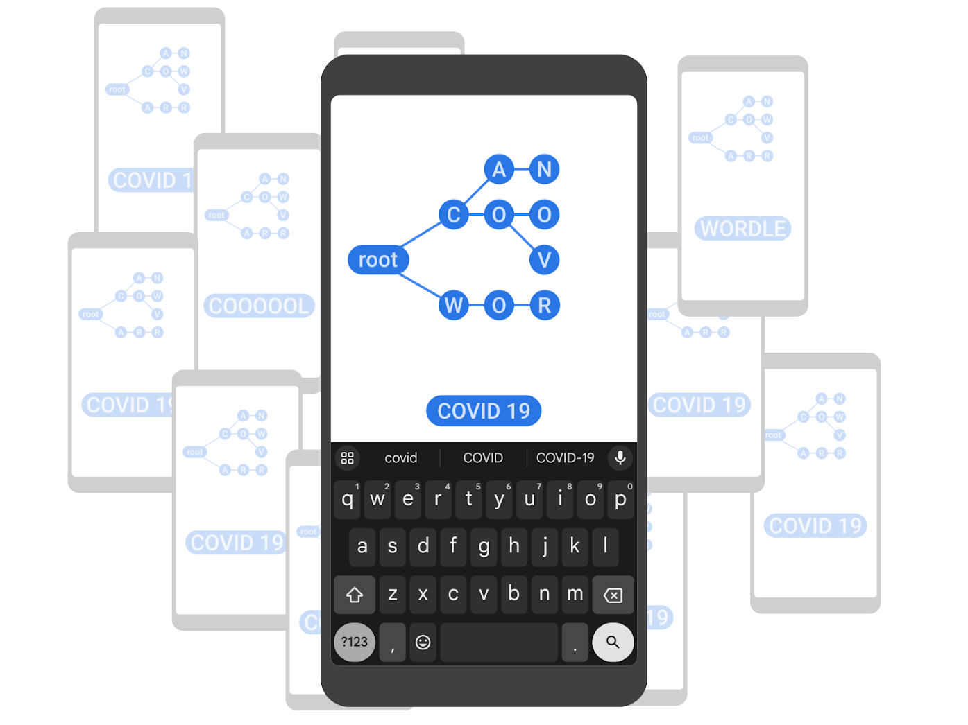
Improving Gboard language models via private federated analytics- Algorithms & Theory ·
- Distributed Systems & Parallel Computing ·
- Product ·
- Security, Privacy and Abuse Prevention
-

April 17, 2024
Robust speech recognition in AR through infinite virtual rooms with acoustic modeling- Human-Computer Interaction and Visualization ·
- Machine Perception ·
- Speech Processing
-
March 18, 2024
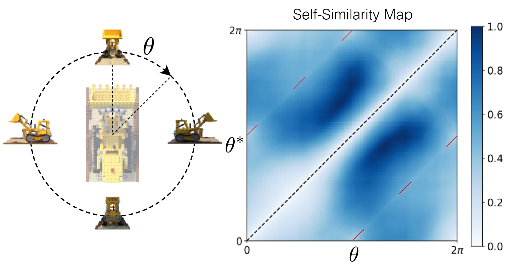
MELON: Reconstructing 3D objects from images with unknown poses- Machine Intelligence ·
- Machine Perception